Chapter 4 Getting work done

4.1.1 Unary operators

To treat a vector or data.table as a set (in the limited sense of dropping duplicates), use unique(x). I guess the function is called “unique” since in the resulting vector (or table), every element (or row) is unique.

For the data.table version, there is a by= option, so we can drop duplicates in terms of some of the table’s columns. By default, it will keep the first row within the by= group, but fromLast = TRUE can switch it to keep the last row instead.

A complementary function duplicated also exists, but is rarely needed.

4.1.2 Testing membership

Besides comparisons, x == y, we can test membership like x %in% y:

c(1, 3, NA) %in% c(1, 2)

# [1]  TRUE FALSE FALSE

"A" %in% c("A", "A", "B")

# [1] TRUE

We get one true/false value for each element on the left-hand side. Duplicate values on the right-hand side are ignored. That is, the right-hand side is treated like a set.

Unlike ==, here we always get a true/false result, even when missing values are present.

4.1.3 Other binary operators

As documented at ?sets, for two vectors x and y we can construct various statements:

• \(x\cup y\) as union(x,y),
• \(x\cap y\) as intersect(x,y),
• \(x\ \backslash\ y\) as setdiff(x,y) and
• \(x = y\) as setequal(x,y).

As mentioned in 2.1.2, R does not actually support an unordered set data type. However, these functions treat x and y as sets in the sense that they ignore duplicated values in them. So union(c(1,1,2), c(3,4)) is c(1,2,3,4), with the repeating 1 ignored because it has no meaning in this context.

Corresponding functions exist for data.tables, prefixed like f*: funion, fintersect, fsetdiff and fsetequal. Two tables can be combined in this way only if their columns line up (in terms of class, etc.).

Looking at the source code for these functions, we’ll see a lot of them use the match function.

4.1.4 Operators on lists of sets

R only includes binary versions of these operators. However, the Reduce function can help for finite unions or intersections. It collapses a list of arguments using a binary operator successively, so the union of four sets

\[ \bigcup_{i=1}^4 x_i = ((x_1\cup x_2) \cup x_3) \cup x_4 \]

is written as

xList = list(1:2, 2:3, 11L, 4:6)
Reduce(union, xList)

# [1]  1  2  3 11  4  5  6

Another alternative for the union of a set of vectors is unique(unlist(xList)). The unlist function just combines the four vectors into a single vector. Reduce(intersect, xList) makes sense for taking the intersection of a bunch of sets.

For a list of data.tables, the same can be done (with funion and fintersect). However, again, the alternative for finite unions unique(rbindlist(dList)) may be better in terms of performance in some cases.

4.1.5 Exercises

1. Define a “subset or equal” function for two vectors, subsetequal(x,y), which returns TRUE iff x is a (nonstrict) subset of y, \(x \subseteq y\). How would the function change for testing a strict subset, \(x \subset y\)?

2. Define a “symmetric difference” function for two vectors, symdiff(x,y), which returns unique items appearing in x or in y but not in both.

3. With DT = data.table(g = c(1,1,2,2,2,3), v = 1:6), we can select the first row of each g group with unique(DT, by="g") or DT[!duplicated(DT, by="g")] or DT[, .SD[1L], by=g] or DT[.(unique(g)), on=.(g), mult="first"] or DT[DT[, first(.I), by=g]$V1]. Find several ways to select the last row in each g group. (Hint: one uses order(-(1:.N)).)

4.2.1 Exercises

1. Define a function, triples, which takes a vector x and returns all length-3 subsets, one on each row. For x = 1:5, there are ten = choose(5,3) such subsets, so it should look something like…

   #     V1 V2 V3
   #  1:  1  2  3
   #  2:  1  2  4
   #  3:  1  2  5
   #  4:  1  3  4
   #  5:  1  3  5
   #  6:  1  4  5
   #  7:  2  3  4
   #  8:  2  3  5
   #  9:  2  4  5
   # 10:  3  4  5

4.3.1 Distribution draws

To draw n random numbers from the uniform distribution on the unit interval, use runif(n). All random-draw functions follow this naming convention – rnorm, rpoisson, rbinom – for a full list of the built-in ones, type ?distributions. Many more are offered in packages that can be found by searching online.

To get a quick look at the density being drawn from, use curve:

# glance at chi-squared with 10 degrees of freedom
df = 10
curve(dchisq(x, df), xlim = qchisq(c(.01, .99), df))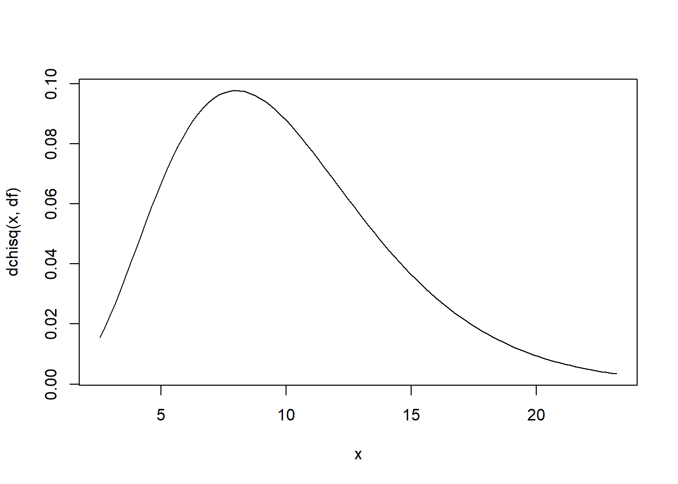

d* is the density and q* is the quantile function. We’re using the latter to find good x-axis bounds for the graph. The final function is p*, for the cumulative density function.

4.3.2 Urn draws

To take n samples from x with replacement, where p[i] is the probability of drawing x[i]:

sample(x, prob = p, size = n, replace = TRUE)

The help page ?sample covers many other use cases. There is one to be very wary of, however:

set.seed(1)
x = c(6.17, 5.16, 4.15, 3.14)
sample(x, 2, replace = TRUE)

# [1] 5.16 5.16

y = c(6.17)
sample(y, size = 2, replace = TRUE)

# [1] 4 6

Where did 4 and 6 come from? Those aren’t elements of y!

I should have instead sampled from ys indices like

y[sample.int(length(y), size = 2, replace = TRUE)]  
# or
y[sample(seq_along(y), size = 2, replace = TRUE)]  

To take draws without replacement, just use the option replace = FALSE.

4.3.3 Permutations

Taking a random permutation of a vector is just a special case of drawing from an urn. We’re drawing all balls from the urn without replacement:

y = c(1, 2, 3, 4)
sample(y) # using default replace = FALSE

The same warning for length-zero or length-one vectors applies here. The safer way is:

y = c(1, 2, 3, 4)
y[sample.int(length(y))]
# or
y[sample(seq_along(y))]

4.3.4 Simulations

For a random process to repeat nsim times, the replicate function is the answer. Suppose we want to take 10 standard normal draws and return the top three:

nsim = 2
n    = 10
set.seed(1)
replicate(nsim, rnorm(n) %>% sort %>% tail(3))

#           [,1]      [,2]
# [1,] 0.5757814 0.9438362
# [2,] 0.7383247 1.1249309
# [3,] 1.5952808 1.5117812

The set.seed line is added so that the results are reproducible.

nsim = 2
n    = 10
set.seed(1)
replicate(nsim, rnorm(n) %>% { list(mu = mean(.), top3 = sort(.) %>% tail(3)) }, simplify = FALSE)

# [[1]]
# [[1]]$mu
# [1] 0.1322028
# 
# [[1]]$top3
# [1] 0.5757814 0.7383247 1.5952808
# 
# 
# [[2]]
# [[2]]$mu
# [1] 0.248845
# 
# [[2]]$top3
# [1] 0.9438362 1.1249309 1.5117812

nsim = 1e4
n    = 1e2
system.time(replicate(nsim, simplify = FALSE,
    rnorm(n) %>% { list(mu = mean(.), top3 = sort(.) %>% tail(3))}
))

#    user  system elapsed 
#    1.55    0.02    1.56

system.time(replicate(nsim, simplify = FALSE, {
    x = rnorm(n)
    list(mu = mean(x), top3 = tail(sort(x),3))
}))

#    user  system elapsed 
#    0.36    0.00    0.35

simparmDT = data.table(set_id = LETTERS[1:2], nsim = 3, n = 10, mu = c(0, 10), sd = c(1, 2))

#    set_id nsim  n mu sd
# 1:      A    3 10  0  1
# 2:      B    3 10 10  2

set.seed(1)
simDT = simparmDT[, .(
    
    # assign a unique ID to each run
    run_id = sprintf("%s%03d", set_id, seq.int(nsim)),  
    
    # run simulations, storing results in a list column
    res = replicate(nsim, simplify = FALSE, {
        x = rnorm(n, mu, sd)
        list(mu = mean(x), top3 = tail(sort(x),3))
    })
    
), by=set_id]

#    set_id run_id    res
# 1:      A   A001 <list>
# 2:      A   A002 <list>
# 3:      A   A003 <list>
# 4:      B   B001 <list>
# 5:      B   B002 <list>
# 6:      B   B003 <list>

sim_fun = function(n, mu, sd){
    x = rnorm(n, mu, sd)
    list(mu = mean(x), top3 = tail(sort(x),3))
}

set.seed(1)
simDT = simparmDT[, .(
    run_id = sprintf("%s%03d", set_id, seq.int(nsim)),  
    res = replicate(nsim, do.call(sim_fun, .SD), simplify = FALSE)
), by=set_id, .SDcols = intersect(names(simparmDT), names(formals(sim_fun)))]

simDT[, (names(simDT$res[[1]])) := res %>% 
    # put non-scalar components into lists
    lapply(function(run) lapply(run, function(x) 
        if (is.atomic(x) && length(x) == 1L) x
        else list(x)
    )) %>% 
    # combine rows into one table
    rbindlist
][]

#    set_id run_id    res         mu                          top3
# 1:      A   A001 <list>  0.1322028 0.5757814,0.7383247,1.5952808
# 2:      A   A002 <list>  0.2488450 0.9438362,1.1249309,1.5117812
# 3:      A   A003 <list> -0.1336732 0.6198257,0.7821363,0.9189774
# 4:      B   B001 <list> 10.2414604    11.52635,12.20005,12.71736
# 5:      B   B002 <list> 10.2682734    11.39393,11.53707,11.76222
# 6:      B   B003 <list> 10.2869137    11.13944,12.86605,13.96080

4.4.1 Lag operators

Data.table provides a convenient tool for the lag operator and its inverse, a “lead operator”:

x = c(1, 3, 7, 10)
shift(x)                # lag

# [1] NA  1  3  7

shift(x, type = "lead") # lead

# [1]  3  7 10 NA

shift(x, 0:3)           # multiple lags

# [[1]]
# [1]  1  3  7 10
# 
# [[2]]
# [1] NA  1  3  7
# 
# [[3]]
# [1] NA NA  1  3
# 
# [[4]]
# [1] NA NA NA  1

shift always returns vectors of the same length as x, which works well with data.tables:

# add to an existing table
DT = data.table(id = seq_along(x), x)
DT[, sprintf("V%02d", 0:3) := shift(x, 0:3)][]

#    id  x V00 V01 V02 V03
# 1:  1  1   1  NA  NA  NA
# 2:  2  3   3   1  NA  NA
# 3:  3  7   7   3   1  NA
# 4:  4 10  10   7   3   1

# make a new table
shiftDT = setDT(c(list(x = x), shift(x, 0:3)))    

#     x V1 V2 V3 V4
# 1:  1  1 NA NA NA
# 2:  3  3  1 NA NA
# 3:  7  7  3  1 NA
# 4: 10 10  7  3  1

The embed function from base R may also be useful when handling lags. It extracts all sequences of a given size:

embed(x, 3)

#      [,1] [,2] [,3]
# [1,]    7    3    1
# [2,]   10    7    3

4.4.2 Taking differences

A simple common use for shift is taking differences across rows by group:

DT = data.table(id = c(1L, 1L, 2L, 2L), v = c(1, 3, 7, 10))
DT[, dv := v - shift(v), by=id]
# fill in the missing lag for the first row
DT[, dv_fill := v - shift(v, fill = 0), by=id][]

#    id  v dv dv_fill
# 1:  1  1 NA       1
# 2:  1  3  2       2
# 3:  2  7 NA       7
# 4:  2 10  3       3

There is also a diff function in base R, but it is less flexible than computing differences with shift; and it does not return a vector of the same length as its input.

4.4.3 Rolling computations

If we want a rolling sum, the naive approach is to take the sum of elements 1:2, then the sum of 1:3, then the sum of 1:4. In the context of data.tables, this would look like a self non-equi join (3.5.7):

# example data
set.seed(1)
DT = data.table(id = rep(LETTERS[1:3], each = 3))[, `:=`(
  sid = rowid(id),
  v   = sample(0:2, .N, replace = TRUE)
)][]

#    id sid v
# 1:  A   1 0
# 2:  A   2 1
# 3:  A   3 1
# 4:  B   1 2
# 5:  B   2 0
# 6:  B   3 2
# 7:  C   1 2
# 8:  C   2 1
# 9:  C   3 1

DT[, vsum := 
  DT[.SD, on=.(id, sid <= sid), sum(v), by=.EACHI]$V1
, .SDcols = c("id", "sid")]

(As a side-note, rowid conveniently builds a within-group counter, as seen here. For more counters, see 4.4.5.)

The number of calculations performed with this non-equi join approach scales at around N^2 as the number of rows N increases, which is pretty poor. Nonetheless, for any rolling computation, this will always be an option.

In this case (and many others), there’s a better way, though:

DT[, vsum2 := cumsum(v), by=id][]

#    id sid v vsum vsum2
# 1:  A   1 0    0     0
# 2:  A   2 1    1     1
# 3:  A   3 1    2     2
# 4:  B   1 2    2     2
# 5:  B   2 0    2     2
# 6:  B   3 2    4     4
# 7:  C   1 2    2     2
# 8:  C   2 1    3     3
# 9:  C   3 1    4     4

Besides cumsum for the cumulative sum, there’s also cumprod for the cumulative product; and cummin and cummax, for the cumulative min and max. For more rollers and to roll new ones, see the zoo and RcppRoll packages.

To “roll” missing values forward, it is common to use na.locf (“last observation carried forward”) from the widely-used zoo package. Alternately, DT[, v := v[1L], by=cumsum(!is.na(v))] can do the trick.

4.4.4 Run-length encoding

In time series, it is common to have repeated values, called “runs” or “spells.” To work with these in a vector, use rle (“run length encoding”) and inverse.rle:

x = c(1, 1, 1, 0, 0, 1, 1, 0, 0, 1, 0, 1, 1, 1)
rle(x)

# Run Length Encoding
#   lengths: int [1:7] 3 2 2 2 1 1 3
#   values : num [1:7] 1 0 1 0 1 0 1

Because the result is a list, we can use with on it (as discussed in the last section). For example, if we just want the final three runs:

r = rle(x)
new_r = with(r, {
  new_lengths = tail(lengths, 3)
  new_values  = tail(values, 3)
  
  list(lengths = new_lengths, values = new_values)
})
inverse.rle(new_r)

# [1] 1 0 1 1 1

As we saw in 2.4.7, with(L, expr) attaches objects in a list or environment L temporarily for the purpose of evaluating the expression expr.

4.4.5 Grouping on runs

cut and findInterval are good ways to construct groups from intervals of a continuous variable.

To group by sequences, it is often useful to take advantage of…

• Cumulative sums: cumsum
• Differencing: diff or x - shift(x), explained in 4.4.1
• Runs: rleid and rle

To label rows within a group, use data.table’s rowid. To label groups, use data.table’s .GRP, like DT[, g_id := .GRP, by=g].

Remember that while it’s often tempting in R to run computations by row, like DT[, ..., by=1:nrow(DT)], this is almost always a bad idea, both in terms of clarity and speed.

4.6.1 Extracting results

The return value from a regression function is a special object designed to hold the results of the run. In the case of a linear regression, the lm function returns a lm object.

To see how this object can be used, look for the object’s attributes and for methods associated with its class:

set.seed(1)
n   = 20
DT  = data.table(
  y = rnorm(n), x = rnorm(n), 
  z = sample(LETTERS[1:3], n, replace = TRUE)
)
res = DT[, lm(y ~ x)]
attributes(res)

# $names
#  [1] "coefficients"  "residuals"     "effects"       "rank"          "fitted.values"
#  [6] "assign"        "qr"            "df.residual"   "xlevels"       "call"         
# [11] "terms"         "model"        
# 
# $class
# [1] "lm"

class(res)

# [1] "lm"

methods(class = "lm")

#  [1] add1           alias          anova          case.names     coerce        
#  [6] confint        cooks.distance deviance       dfbeta         dfbetas       
# [11] drop1          dummy.coef     effects        extractAIC     family        
# [16] formula        hatvalues      influence      initialize     kappa         
# [21] labels         logLik         model.frame    model.matrix   nobs          
# [26] plot           predict        print          proj           qr            
# [31] residuals      rstandard      rstudent       show           simulate      
# [36] slotsFromS3    summary        variable.names vcov          
# see '?methods' for accessing help and source code

Attributes can always be accessed like attr(obj, attr_name); while some have their own accessors, like coefficients(res). Methods are functions that can be applied directly to the object, like plot(res, 1). For documentation on methods, add a dot and the class, like ?plot.lm and ?predict.lm.

Besides usage like DT[, lm(y ~ x)], most regression functions also offer a data argument, like lm(y ~ x, data = DT).

4.6.2 Formulas

The y ~ x expression above is called a formula. These can greatly simplify the specification of a regression equation.

For example, if we want the categorical variable z on the right-hand side, there is no need to construct and list a set of dummies (as noted in 3.8.3):

lm(y ~ z, data = DT)

# 
# Call:
# lm(formula = y ~ z, data = DT)
# 
# Coefficients:
# (Intercept)           zB           zC  
#      0.5265      -0.6201      -0.4283

And there are many other simple extensions:

# including all levels of z by dropping the intercept
lm(y ~ z - 1, data = DT)

# 
# Call:
# lm(formula = y ~ z - 1, data = DT)
# 
# Coefficients:
#       zA        zB        zC  
#  0.52645  -0.09363   0.09816

# including an interaction term
lm(y ~ z:x, data = DT)

# 
# Call:
# lm(formula = y ~ z:x, data = DT)
# 
# Coefficients:
# (Intercept)         zA:x         zB:x         zC:x  
#     0.20267     -0.25431     -0.46956     -0.07843

# including all of z's levels by dropping x and the intercept
lm(y ~ z*x - 1 - x, data = DT)

# 
# Call:
# lm(formula = y ~ z * x - 1 - x, data = DT)
# 
# Coefficients:
#       zA        zB        zC      zA:x      zB:x      zC:x  
#  0.46634  -0.02306   0.10293  -0.18133  -0.25044  -0.06683

# including a polynomial
lm(y ~ poly(x, 2), data = DT)

# 
# Call:
# lm(formula = y ~ poly(x, 2), data = DT)
# 
# Coefficients:
# (Intercept)  poly(x, 2)1  poly(x, 2)2  
#      0.1905      -0.8659       2.3428

The doc at ?formula explains all the ways to write formulas concisely. Many functions besides lm allow the same sorts of formulas.

We saw dcast (3.7.6) also uses formulas. These only come in very simple forms, as documented in ?dcast.

4.6.3 Custom regression

If no one has implemented the regression procedure we want, it is possible to program up a basic version of it (assuming we understand it). Writing up a version that works nicely with formulas and has all the attributes and methods seen with lm would be a tall order, of course.

It’s best for speed and simplicity to lean on matrix algebra as much as possible. If speed becomes a real issue, translating to C++ with the Rcpp package may help.

4.7.1 Optimization

To find an extremum of a function of a length-one number (a real scalar), use optimize. For functions of multiple arguments, there’s optim. (R is agnostic on Brit vs American English, so optimise does the same thing as optimize.)

The documentation covers everything (optimization methods available, numerical issues to be aware of, stopping rules, “trace” options).

4.7.2 Integration

Given a vectorized function (2.3.4) mapping to and from the real line and an interval, integrate will approximate the associated definite integral. The documentation explains the method used and the numerical issues.